Quick Solutions to Solve SPICE Convergence Issues.

This article delves into the critical subject of to Solve SPICE Convergence Issues. The solutions presented for addressing convergence issues are of a general nature and are applicable across various algorithms, such as PSPice, XSPICE, NGSPICE, IsSPICE, and HSPICE. By understanding and effectively managing convergence challenges in SPICE simulations can enhance the reliability and accuracy of their electronic circuit analyses, regardless of the specific SPICE variant they are utilizing.

Convergence problems in SPICE simulations primarily manifest in three distinct categories:

  • Circuit Topology Errors

The SPICE simulation software frequently signals these types of errors with precise messages, rendering their identification and rectification relatively straightforward.

  • SPICE simulator Options Settings

For instance, during transient analysis, selecting an appropriate timestep corresponding to the device’s operational frequency becomes very important. At times, a compromise between accuracy and convergence stability is required; as accuracy is increased, the likelihood of encountering convergence errors also rises.

  •  Unrealistic SPICE models

Convergence problems can stem from SPICE models characterized by significant nonlinearities and discontinuities. Such models introduce complexities that can challenge the simulation’s convergence process.

Advanced SPICE options window in PSpice

Now, let’s delve into the strategies that swiftly address the most prevalent convergence challenges arising from these distinct problem categories in order to effectively solve SPICE convergence issues.

Circuit Topology Errors

Ground Absence, Error Message: Node is Floating.

The SPICE algorithm computes voltage for every circuit point relative to a reference point—this reference point is specifically the ground, an essential component in the circuit. Including the ground reference wherever needed suffices to address this issue.

Lack of Direct DC Ground Path, Error Message: Node is Floating.

Building on the insights from the prior scenario, it’s essential to verify the absence of circuit points isolated from the ground reference. If an apparent isolation is intended for a node from the ground, this can be achieved by introducing a high-value resistor that ensures continuity with the ground reference. Ensure that the node maintains a direct connection with the ground reference.

Unmodeled pins, error message: Less than two connections at node

This error emerges when the Capture component lacks an associated SPICE model or when a wire is “floating,” connected to a device pin without a corresponding connection to another pin.

Prevent Loops Involving Voltage Sources or Inductors, Error Message: Voltage Source or Inductor Loop

A potential solution involves incorporating a minor series resistance.

Avoid series capacitors or current sources

Ensure the absence of series capacitors or series current sources.

Convergence Problems due to SPICE Simulation options settings

Primarily, it’s crucial to establish a suitable timestep corresponding to the device being simulated. For instance, if we intend to simulate a 1 kHz oscillator with a period of T=1 ms, it’s advisable to configure a timestep on the order of T/10 or even lower. This ensures a satisfactory simulation resolution.

Let’s categorize the solutions applicable to the two principal types of analysis: DC and Transient. Notably, once DC convergence is achieved, the AC analysis will also converge.

Solve SPICE convergence issues for DC Analysis

ITL1: set ITL1=500, this set iterations limit that SPICE will perform for DC and bias.

ITL2: set ITL2=500, this set iterations limit that SPICE will perform for DC and bias before giving up.

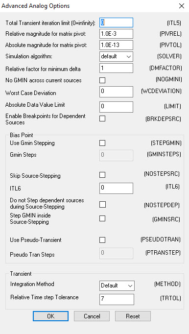
ITL6: set ITL6=100 (Advanced Options), this increases Source stepping iteration limit, Default value
is 0, which disables source stepping.

Reduce ABSTOL Absolute current tolerance, it should be set to about 8 orders of magnitude below the level of maximum current, the dafault value is 1pA

Diminish VNTOL Absolute voltage tolerance, as for ABSTOL it should be set to about 8 orders of magnitude below the level of maximum voltage, the default value is 1uV

Modify RELTOL this is the relative error allowed for node voltage and branch current. Set RELTOL= 0.01 to reach a compromise between accuracy and simulation run time. The default value is 0.001.

GMIN set GMIN = 1n or 0,1n. GMIN is the minimum conductance across all semiconductor devices

GMINSTEPS (Advanced Options) set GMINSTEPS=200 . This option adjusts the number of increments for GMIN during the DC analysis.

Change DC Power supplies into Pulse generator

NODESETs use .NODESETs statement to assign a voltage to a node. This can be done for example when the node-voltage table shows unrealistic voltages. If it’s not available a proper estimation of the node DC voltage, use a .NODESET of 0V.

Solve SPICE convergence issues for Transient Analysis

RELTOL also for the transient analysis Set RELTOL= 0.01 (The default value is 0.001), that decreases the accuracy
of the simulation by increasing the error tolerance required for convergence.

ITL4 set ITL4=2000 , this increases the number of iterations before a nonconvergence warning is issued

reduce ABSTOL Absolute current tolerance, it should be set to about 8 orders of magnitude below the level of maximum current, the dafault value is 1pA

Reduce VNTOL Absolute voltage tolerance, as for ABSTOL it should be set to about 8 orders of magnitude below the level of maximum voltage, the default value is 1uV

ITL5 set ITL5=0 that assigns infinity to the total transient iteration limit.

Reduce rise and fall of PULSE sources

GEAR (Advanced Options) Select METHOD=GEAR, this is the integration method that SPICE uses to solve transient equations. Very useful for oscillators and switching circuits SPICE simulations.

TRTOL set TRTOL=40. this is the tolerance for integration error calculated using transient analysis. The TRTOL
value should NOT be greater than 1/RELTOL. the default value is 7.

IC set Initial conditions for the capacitors at their expected operating voltage. Setting this data causes
SPICE to bypass the DC operating point analysis.

Utilize Reliable SPICE Models.

It’s essential to acknowledge that SPICE models do not perfectly mirror the devices they represent; rather, they offer a partial depiction. SPICE models featuring pronounced non-linearities or abrupt discontinuities have the potential to trigger substantial convergence difficulties.

These abrupt shifts might stem from the exclusion of certain device behaviors, such as parasitic elements like capacitance across all semiconductor junctions, stray capacitance, and RC snubbers encircling diodes. In most instances, it’s advisable to rely on vendor-released SPICE models. However, if directly modeling the device, it becomes imperative to diligently mitigate any sources of discontinuities and non-linearities to ensure smoother operation.

SPICE Simulation Libraries:

On this page, you can find libraries of SPICE models for various components, released by major electronic device manufacturers.

Reference:

EMA Design Automation Resolving Simulation Errors
SPICE Circuit Handbook Steven. M Sandler Charles Hymowitz

Design the Loop Controller for Switching Power Supplies.

Ing. Cristoforo Baldoni

Switching power supplies loop controller design: In this article, we will explore the process of determining the output power stage transfer function H(s), also known as the Control-to-Output function, for different types of switching power supplies is the focus of this article. We’ll delve into BUCK, BOOST, BUCK-BOOST, HALF-BRIDGE, and FULL BRIDGE configurations under both voltage mode control and current mode control. Despite the intricate nature of various power supply variants that incorporate one or more output feedback mechanisms, the output power transfer function H(s) can be categorized into schematic classifications of general applicability.

We will also examine scenarios wherein it becomes necessary to consider the influence of the Right Half Plane Zero (RHPZ) and the practical implications it entails. Once the components specific to the particular power supply are appropriately dimensioned, we can reasonably approximate the transfer function that mathematically describes the output power stage. As highlighted in the article “Find Poles and Zeros of a Circuit by Inspection“, will promptly identify the POLES and ZEROS characterizing the distinct switching categories.

The subsequent step involves generating Bode plots of these functions utilizing PSpice. Based on their characteristics, we will select the most suitable compensator G(s), implementing the compensation network through operational amplifiers integrated within the microcontrollers. Employing SPICE simulation on the open loop transfer function G(s)*H(s), we can assess the system’s stability outcomes.

Lastly, we will apply this methodology to two real-world switching power supply instances: a low-power flyback converter and an off-line, half-bridge switching configuration. This approach streamlines the design process for the compensator G(s) during the prototyping phase, preceding physical measurements with instrumentation.

It’s strongly recommended to read these articles first:

By accessing this article, you can download the following SPICE simulation files related to the design of compensation for switching power supplies:

-Forward function example

-Flyback function example

-Flyback function example with a Right Half Plane ZERO

-Origin POLE compensator

-Origin POLE Transfer function implementation

-Forward function compensated example

-One ZERO two POLES compensator

-One ZERO two POLES Transfer Function Implementation

-Flyback with RHPZ compensated

-Three POLES two ZEROS compensator

-Three POLES two ZEROS Transfer Function

-Transfer function of a real Flyback converter

-Compensator for the flyback converter

-Overall compensated  transfer function of the flyback converter

-Transfer function of a real Forward converter

-Compensator for the Forward converter

-Transfer function of compensator for the Forward converter

-Overall compensated  transfer function of the Forward converter

Premium Content

Login to buy access to this content

Combination Wave Generator SPICE simulation.

In this article, we will delve into the implementation and analysis of a versatile Combination Wave Generator SPICE simulation template. This template forms the groundwork for a range of applications including Surge Generators, Line Impedance Stabilization Networks (LISN), motor control, and ripple current analysis. Hardware engineers can capitalize on this model to streamline project development efforts.While using PSpice for simulation, you can effortlessly apply the fundamental principles of the Combination Wave Generator SPICE simulation template to various other SPICE simulation software platforms.

A “Combination Wave Generator” finds its application in Electromagnetic Compatibility (EMC) tests, generating specific waveform voltage or current pulses. Its purpose is to assess electronic devices’ electrical resilience and responses to abrupt variations or transients within the electromagnetic environment. These generators replicate transient electrical disruptions or surges that might manifest in electronic circuits during situations like electrostatic discharges, switching transients, or line surges.

The Combination Wave Generator is an essential component of EMC compliance tests, ensuring that electronic devices can operate in realistic electromagnetic environments without sustaining damage or unforeseen behaviors.

Simplified SPICE Model of Combo Wave Generator.

The simplified model of the CWG consists of an High-Voltage source U, a charging resistor Rc, an energy storage capacitor Cc. This part of circuit is connected by a switch to 2 Pulse duration shaping resistors Rs, an impedance matching resistor Rm and a Rise time shaping indutor Lr, as in the picture below


GPM-SurgeGenerator_page3_image1


typical values of this components are:  Cc=7.76μF,  Rs1=14.8 Ohm,  Rm=1.05 Ohm,  Lr=9.74μH,  Rs2=23.3 Ohm. The peak voltage on Rs2 can be 1KV, 2KV,..6KV.

In the following schematic we set the high voltage with the initial condition of the CapacitorCc, for example for 6KV, we set 6300 in the PSpice IC field of the Cc component. We can adjust the time in U1 to make surge hit at 90/270 degree or whatever phase we want.


GPM-SurgeGenerator_page4_image1
GPM-SurgeGenerator_page4_image2


Calibration of Surge Generator.

The IEC/EN 61000-4-5 standars requires the following waveform of open-circuit voltage with no Coupling/Decoupling network (CDN) connected


GPM-SurgeGenerator_page5_image1


This is the result of the simulation that shows a voltage waveform that fullfills requirementof IEC/EN 61000-4-5

GPM-SurgeGenerator_page5_image2


Below the image of the waveform of short-circuit current with no CDN connected

GPM-SurgeGenerator_page6_image2


and here again the simulated results:


GPM-SurgeGenerator_page6_image1


Ipeak is about 1.5KA, T1 is 8uS and T2 is 20uS. The effective coupling impedance is 2Ohm. The simulated current waveform fulfills requirement of IEC/EN 61000-4-5 standards.

Microcontroller-Based PID Controller Design and Simulation.

Ing. Cristoforo Baldoni

In this article, we will explore the transition from analog PID controller design for continuous-time systems to digital controllers, including PID controller simulation. This transition involves substituting operational amplifiers, resistors, and capacitors with microcontrollers. Digital controllers offer remarkable compactness, fitting the entire controller onto a single chip, complete with A/D and D/A converters. Furthermore, digital controllers remain immune to component aging and temperature-induced value fluctuations, in contrast to analog components.

We will delve into the application of the Z-transform, which serves as the discrete-time systems counterpart to the Laplace transform. This exploration will encompass the identification of a process’s transfer function. Through a systematic, step-by-step approach, we will demonstrate the practical application of theoretical insights. This will be accomplished by analyzing a Proteus microcontroller-based project, wherein the PWM output is harnessed to regulate the temperature of an oven. The microcontroller boasts a 10-bit A/D converter.

This adaptable procedure can be easily customized with minimal adjustments for controlling various other processes.

Topics Covered:

1. Digital Control-System Block Diagrams.

2. Linear Difference Equations, Z-Transform, Inverse Z-Transform and Discrete Transfer Function.

3. Sampling and A/D Conversion: Analog to Digital Converter.

4. D/A Conversion and ZERO ORDER HOLD  (ZOH) : Relationship between the Continuous Transfer Function and Discrete Transfer Function of a Sampled Process.

5.  Manipulation of Block Diagrams for Sampled Data.

6. Methods for designing Digital Controllers and Ensuring Stability.

7. Microcontroller-Based PID Controller Design.

8. Transfer Function Identification and PID Tuning using the Ziegler–Nichols Method.

9. Practical case of a temperature control system implemented with a microcontroller PIC and simulated with ISIS Proteus: Step by step explanation of how to apply the theoretical knowledge for implementing and simulating a PID controller.

Premium Content

Login to buy access to this content

Find Poles and Zeros of a Circuit by Inspection

 Ing. Cristoforo Baldoni

In this article, focused on ‘Poles and Zeros of a Circuit‘, we will explore the technique of identifying the count of poles and zeros within a transfer function, including those in complex linear networks, solely through visual inspection. This method obviates the need for calculating the analytical expression of the transfer function. By the conclusion of this article, you will have the capability to swiftly determine the number of poles upon initial examination.

Once the output is established, this approach also enables you to ascertain the quantity of zeros through inspection and subsequently compute the precise symbolic form of the transfer function. Additionally, you can calculate the exact values of both zeros and poles employing user-friendly software tools readily accessible for free. We will validate the findings using SPICE analysis.

The primary objective of this article is to delve into the concepts of poles and zeros within a transfer function, elucidating their physical significance. Furthermore, we aim to furnish valuable analytical tools to aid analog circuit designers and control systems engineers in their endeavors.

How many POLES does this circuit have?

polesnetworkBig

And how many does this high-pass filter have?

fiveorderHPfilter

If your response to the initial question is 9 or 8, or if you do not identify a fifth-order filter (with five poles) in the filter’s illustration, then you should proceed to read this article.

Premium Content

Login to buy access to this content

Getting Started with PyOPUS

PyOPUS is a Python based platform for very sophisticated circuit optimization and simulation automation. It represents a library designed for optimizing arbitrary systems through simulation. Its primary focus is on refining circuit performance. Serving as the foundation for the PyOPUS GUI, this library facilitates the effortless configuration of design automation tasks. Within the GUI, users are also able to visualize outcomes and graph the waveforms produced by the simulator.

The module labeled “pyopus.simulator” presently offers compatibility with SPICE OPUS, Ngspice, Xyce, HSPICE, and SPECTRE. The use of the Python library with the simulator requires a previous SPICE OPUS (or other SPICE software compatible) installation, then refer to the relative tutorial before proceeding.

Now let’s see how to install PYOPUS on Windows. The download page offers software for Linux and Windows platforms, but discontinues 32-bit Windows support due to the unavailability of the 32-bit Windows SciPy wheel.

Python Programming language
NumPy Package for scientific computing with Python
SciPy Python software for mathematics, science, and engineering
MatPlotLib Python 2D plotting library
wxPython Blending of the wxWidgets C++ class library with Python
PyOPUS installerthe Windows PyOPUS installer

All these softwares can be downloaded here

Let’s start with the Python installation


the default destination directory is C:Python26


the full features installation requires about 50MegaByte


after the installation we have to add an enviroment variable: Start/Control Panel/System and Security/System/Advanced system settings, now click on Enviroment Variables button.


add to “Path” variable the value “C:Python26”


SPICE OPUS Circuit Simulation

SPICE OPUS, an acronym for SPICE engine for OPtimization UtilitieS, represents a powerful circuit simulation tool. This software is a recompilation of the original Berkeley’s source code, designed to work seamlessly on Windows 95/98/NT and Linux operating systems, supplemented by Georgia Tech Research Institute’s XSPICE mixed-mode simulator.

With SPICE OPUS, you have the capability to perform simulations on a wide range of circuit types, including analog, digital, and mixed-signal configurations. This versatile tool is available for both Windows and Linux platforms, although it does not feature an integrated schematic program for component selection and circuit drawing.

Developed by the Faculty of Electrical Engineering at the University of Ljubljana, Slovenia, SPICE OPUS has gained substantial recognition worldwide, amassing a user base of over 10,000 individuals spanning various domains such as research, education, and industry.

Throughout this article, we will guide you through the straightforward process of installing SPICE OPUS on a Windows environment. Additionally, we’ll delve into the procedure for describing a circuit to simulate, achieved by crafting a .cir file using a standard text editor.

You can download the updated software here

After downloading the program run the Setup.exe

Installation on Windows


you can change the installation directory by clicking on Browse button, by default it is installed in C:SpiceOpus


when the setup is complete, open the Start menu and go to Control Panel, choose “System and Security” and again “System”, once open this window,  click on “Advanced system settings”


the “System Properties”  window pops up:


click on “Enviroment Variables…”


Add a new system variable by clicking on the lower “New” button.

Name the variable OPUSHOME. The specified directory must be the Spice Opus installation directory. Click on OK. Confirm your changes by clicking on OK in the Environment variables dialog and once more in the

System Properties dialog.


Installation on Linux

Become root.

su –

Unpack the .tar.gz archive.

A directory will be created with the name that looks like

spice_opusXXX_linux_DATE_TIME

Enter this directory.

cd spice_opusXXX_linux_DATE_TIME

Start the installation script (spice.install).

./spice_install INSTALL_PREFIX

INSTALL_PREFIX is the tree where Spice Opus will be installed. The recommended location is

/usr/local. The installation script removes any previous Spice Opus installation in that tree and

replaces it with the latest version. The binaries go to INSTALL_PREFIX/bin .

After the installation is finished, you can remove the spice_opusXXX_linux_DATE_TIME

directory that was created by unpacking the .tar.gz archive.

Setting up the environment.

We shall assume that you are using BASH. Add the following two lines to /etc/profile (you

must be root in order to be able to do it).

OPUSHOME=INSTALL_PREFIX

export OPUSHOME

where INSTALL_PREFIX is the tree where you installed Spice Opus.

It is also convenient if you add INSTALL_PREFIX/bin to your path. Add the following two

lines at the end of /etc/profile.

PATH=$PATH:$OPUSHOME/bin

export PATH

Log out and log in again for the changes to take effect.

TINA spice simulation

TINA SPICE Simulation

TINA is a versatile and user-friendly software tool that empowers users to design, simulate, and optimize electronic circuits with precision and efficiency. Its extensive feature set and TINA SPICE simulation capabilities make it a valuable resource in the field of electronics design and analysis. Here are some key characteristics of TINA:

  1. Intuitive User Interface: TINA boasts an intuitive and user-friendly interface, making it accessible to both beginners and experienced users. Its drag-and-drop functionality and interactive components simplify the process of designing and simulating circuits.
  2. Extensive Component Library: TINA provides an extensive library of electronic components, including semiconductors, passive components, and specialized devices. This library allows users to quickly build complex circuits by selecting and configuring components.
  3. SPICE Simulation Engine: TINA is powered by a robust SPICE (Simulation Program with Integrated Circuit Emphasis) simulation engine. This engine accurately models the behavior of electronic components and circuits, enabling users to predict how their designs will perform in the real world.
  4. Mixed-Signal Simulation: TINA supports mixed-signal simulation, allowing users to design and analyze circuits that combine analog and digital components. This is particularly useful for designing integrated systems.
  5. Parameter Sweeps and Optimization: Users can perform parameter sweeps and optimization studies to explore different design scenarios and find the optimal values for circuit parameters. This feature helps in fine-tuning designs for specific requirements.
  6. Interactive Waveform Analysis: TINA offers advanced waveform analysis tools that allow users to examine voltage and current waveforms at various points in the circuit. This helps in identifying and troubleshooting issues in the design.
  7. Interactive 3D PCB Design: TINA includes a 3D PCB design module that enables users to create and visualize printed circuit boards. This integration streamlines the transition from schematic design to PCB layout.
  8. Educational Resources: TINA is often used in educational settings due to its educational versions and resources. It provides a practical platform for learning electronics and circuit design principles.
  9. Integration with Microcontrollers: TINA can interface with various microcontrollers, making it suitable for embedded systems design. Users can simulate the interaction between microcontrollers and external circuitry.
  10. Custom Component Creation: For unique or specialized components, TINA allows users to create custom models, ensuring accurate simulation results for specific components or devices.

In this initial undertaking, we will commence our initial endeavors with TINA SPICE Simulation by formulating a three-stage BJT audio amplifier circuit. This preliminary endeavor aims to demonstrate the functionality of TINA while concurrently establishing a substantial groundwork for comprehending the complexities associated with electronic circuit design and simulation. Thus, we shall proceed to investigate the captivating domain of electronic design with TINA SPICE Simulation.

To delve deeper into the software’s features, you can refer to this article.


After running the program, we can see this window:


Globalview


On the components toolbar, there are devices in the ‘basic’ tab. Below the toolbar, when you select ‘semiconductors’ on the toolbar, several types of semiconductors appear:


Now select “Special”


And once again, we have a large number of devices to choose from. Let’s begin by selecting a resistor:


Place Resistors, to set value, double-click on one, and a parameters window will appear


Keep the libraries ordered

Learn to design a circuit with PSpice is a task quite simple and is enough a few pages of any manual available on line to do it. What can be confusing is the number of files with different extensions that belong to this great tool of electronic simulation. This is due to the history of PSpice, which initially developed to be used in PC by Microsim passed after to OrCAD which was at last acquired by Cadence. The original CAD Microsim was Schematics. After, the program was provided with a design tool more advanced, Capture, maintaining the ability to still use Schematics.

Schematics image:


Capture image:


Fortunately, the syntax used to describe a component remained the same, and all libraries with mathematical models, are the . LIB. Creating the design of a circuit with PSpice Schematics, the project will be composed of a schematic file .SCH, a control file .CIR and a circuit description file .NET both automatically generated from Schematics, and files .INC containing subcircuits, to be included in the project. The libraries containing the mathematical models to be added to the project are always .LIB, while libraries that contain graphic symbols associated with the mathematical models are the .SLB.

By using the tool of OrCAD Capture, the main project file becomes the .OPJ, and symbolic libraries are now .OLB. In short, in Schematics a component is completely defined by libraries .LIB and .SLB while in OrCAD Capture by the couple .LIB an .OLB.

Currently most of designers use OrCAD Capture for the circuits design, however, the same Capture has a tool to convert project designed with Schematics and convert .SCH and .SLB in .OPJ and .OLB. We ‘ll see how in a dedicated article.

SPICE Simulation Software

SPICE Simulation Software

Exploring the World of SPICE Simulation Software: A Comprehensive Overview

In the field of electronics design and analysis, SPICE (Simulation Program with Integrated Circuit Emphasis) software plays a crucial role in predicting circuit behavior, optimizing designs, and identifying potential issues before costly prototyping or production. This article will provide a comprehensive overview of various SPICE simulation software, encompassing both free and commercial options, along with their distinctive features and capabilities.

LTspice: Engineered by Linear Technology (now Analog Devices), LTspice stands as a widely acclaimed and potent free SPICE simulator. It delivers an intuitive interface, rendering it apt for novices and experienced professionals alike. Its extensive component repository, encompassing numerous Analog Devices components, guarantees precision in simulations. Moreover, LTspice permits users to craft bespoke models, conferring a high degree of versatility across a myriad of electronic circuits.

KiCad: KiCad, an open-source electronics design automation suite, houses an inherent SPICE simulator named NgSpice. This complimentary tool proves particularly valuable for seamless integration with KiCad’s schematic capture and PCB layout attributes. KiCad’s NgSpice bestows a comprehensive array of simulation choices, spanning AC, DC, transient, and more intricate analyses. It finds favor among hobbyists, students, and small-scale ventures.

TINA-TI: Forged by Texas Instruments, TINA-TI is a user-friendly and robust commercial SPICE simulator. While a free version (TINA-TI Webench) exists, the complete iteration features advanced functionalities, aligning with professional engineers and expansive projects. TINA-TI flaunts an expansive component repository, encompassing diverse Texas Instruments devices, ensuring accurate circuit modeling and analysis.

PSpice: Hailing from Cadence Design Systems, PSpice is a versatile and widely employed commercial SPICE simulator. It caters to both analog and mixed-signal simulations, rendering it suitable for intricate circuits. PSpice’s distinctive Sensitivity and Monte Carlo analyses aid in gauging circuit performance across diverse scenarios. Its extensive library of manufacturer-specific models guarantees seamless correspondence with real-world components.

SIMetrix/SIMPLIS: SIMetrix, a commercial SPICE simulator, prioritizes swift and precise simulations, catering to both analog and mixed-signal circuits. Its user-friendliness and compatibility with standard SPICE models render it a favored choice among design engineers. Meanwhile, SIMPLIS, nestled within SIMetrix, excels in switch-mode power supply (SMPS) and control loop simulations, presenting efficient designs for power electronics applications.

Altium Designer: Altium Designer stands as a holistic PCB design software, boasting an inherent SPICE simulator. It presents a seamless design flow, intertwining schematic capture, PCB layout, and simulation. The interface’s intuitiveness, coupled with advanced simulation capabilities, positions Altium Designer as a preferred solution among professional electronic designers.

ICAP/4: Intusoft’s ICAP/4 is a robust SPICE simulator renowned for its precision and accuracy. It spans an extensive spectrum of circuit types, encompassing analog, digital, and mixed-signal designs. ICAP/4’s comprehensive device model repository ensures faithful representation of various components in simulations.

5Spice: As a user-friendly and economical SPICE simulator, 5Spice finds suitability in educational endeavors and compact projects. Despite its cost-effectiveness, 5Spice endows a comprehensive array of simulation features, endowing it with immense value for electronics enthusiasts and students.

Proteus: Heralding from Labcenter Electronics, Proteus stands as a professional electronics design software, harboring a formidable SPICE simulator. It furnishes an amalgamated milieu for schematic capture, PCB layout, and simulation. The advanced simulation choices within Proteus cater to both analog and digital circuits, rendering it a staple among engineers and researchers.

NI Multisim: The brainchild of National Instruments, NI Multisim emerges as a user-friendly and feature-rich SPICE simulator. It unveils an expansive component repository and seamless compatibility with other NI products, affording an extensive domain for electronic design analysis and validation.

TopSpice: Emerging as a versatile commercial SPICE simulator with advanced modeling capabilities, TopSpice thrives in complex electronic systems. Its manifold simulation options facilitate meticulous analysis of circuits under diverse operational contexts.

Micro-Cap: As a comprehensive SPICE simulator prioritizing analog and mixed-signal simulations, Micro-Cap’s user-friendliness and robust simulation engine earn it acclaim among design engineers and researchers.

Spice Opus: Spice Opus assumes the form of an open-source SPICE simulator, tailored for efficient and precise circuit simulations. Its adaptability and alignment with standard SPICE models mark it as a coveted resource for electronics aficionados and researchers.

ViaDesigner Suite: Encompassing an integrated electronics design software boasting a SPICE simulator, ViaDesigner Suite weaves a complete solution for circuit design, simulation, and PCB layout. This comprehensive approach positions it as the preferred choice for seasoned designers.

EDWinXP: EDWinXP stands as an all-encompassing electronics design suite, coupling with a SPICE simulator. It caters to a diverse landscape of electronic designs, unveiling seamless amalgamation and efficient simulation capabilities.

In Conclusion:

The choice of SPICE simulation software hinges upon specific project requisites, budget considerations, and circuit intricacies. Whether one’s preference gravitates toward gratis tools like LTspice and KiCad’s NgSpice, or commercial titans such as TINA-TI, PSpice, SIMetrix/SIMPLIS, Altium Designer, or any of the other aforementioned software, these instruments empower designers to dissect and optimize electronic circuits, ultimately propelling innovation and dependability within the electronics sphere.


CompanySPICE softwareImagesoftware license
AltiumAltium DesigneraltiumdesignerCommercial
KiCadKiCadKiCadFree
cadencelogoCadence OrCAD SolutionsOrCADSoftwareCommercial
designsoftlogoTINA Design SuiteTINAcalculatorCommercial
5Spice5Spice5SpiceProCommercial
intusoftlogoICAP/4 icapsoftwareCommercial
labcenterlogoProteus proteussoftwareCommercial
lineartechnologyLTSpice IVltspicesoftwareFree
nationalinstrumentsNI Multisim MultisimCommercial
penzarlogoTopSpicetopspiceCommercial
spectrumlogoMicro-Cap Micro-CapFree
logoOpusSpiceSpice OpusspiceopusFree
triadsemilogoViaDesigner SuiteViaDesignerFree
visionicsEDWinXPedwinxpCommercial


SPICE Libraries Models:

On this page, you will find links to the SPICE model libraries of various electronic components from major manufacturers.